The EMA workbench: using parameter ranges to reduce uncertainty in LCA modeling
There is always a degree of uncertainty to the input data used in LCA models. Not every value or process is known, so doing an LCA always involves a certain level of guessing, which results in uncertainty in the outcomes. To make sure you can still draw conclusions from your LCA, an uncertainty assessment is a good idea – it shows how much influence certain assumptions have on the outcome and helps correct for that, for instance by expressing the results in a range rather than a value.
Uncertainty is not just lurking in the background
The Wiedema and Wesnæs’s pedigree matrix is a well-known way to do uncertainty analysis: judging data according to its reliability, completeness, and temporal, geographical and technological differences. This type of analysis is great for looking at background data – data about processes over which decision-makers have no direct control (for instance the emissions of the electricity you use). However, there is no well-defined uncertainty assessment for foreground data (the decisions under your control, such as which plastics to use in manufacturing). The exploratory modelling and analysis (EMA) workbench might fill this gap.
Assessing uncertainty by checking many scenarios
The EMA workbench is a computational experimenting tool that allows you to run thousands of scenarios automatically, analyzing how the uncertainty in input parameters causes uncertainty in the outcomes of model scenarios. Instead of having to enter inputs manually for each scenario, the EMA workbench allows you to specify a range of inputs. The tool then generates the results of those multiple scenarios automatically. The EMA workbench also has built-in features for analyzing these results, facilitating a means for the interpretation of results.
The EMA workbench can be used both with simple cases and with complex LCA models. A great feature is optimization of a scenario within certain constraints. For instance, if the environmental impact of a product has to be less than a certain value, that can be provided as a constraint. The EMA workbench can then provide a range of input values that will give results below the limit you entered.
Two-step uncertainty analysis
In the EMA workbench, an uncertainty analysis consists of two phases.
- Experimentation: Setting up estimated ranges for uncertain parameters, both those that are and those that are not under the control of decision-makers. This phase also specifies the total number of times the model is to be run. In a single model run, the tool selects parameter values from the specified ranges and computes the results. The model is then re-run using a different set of parameter values from within the uncertainty range. This is repeated until all parameter ranges have been covered.
- Analysis: Once all model runs are complete, the tool shows the results and starting parameter for each model run. For an LCA model, these model results could be the environmental impact of different impact categories. The EMA workbench has in-built functions for analyzing the results, such as feature scoring, scenario discovery, pair plots, and sensitivity analysis. These functions give the user valuable insights. For instance, feature scoring can be used to identify the relative importance of input parameters on the model results, while scenario discovery can be used to identify the input parameter space that results in the best or worst model results.
Solar panels on residential rooftops: a case study
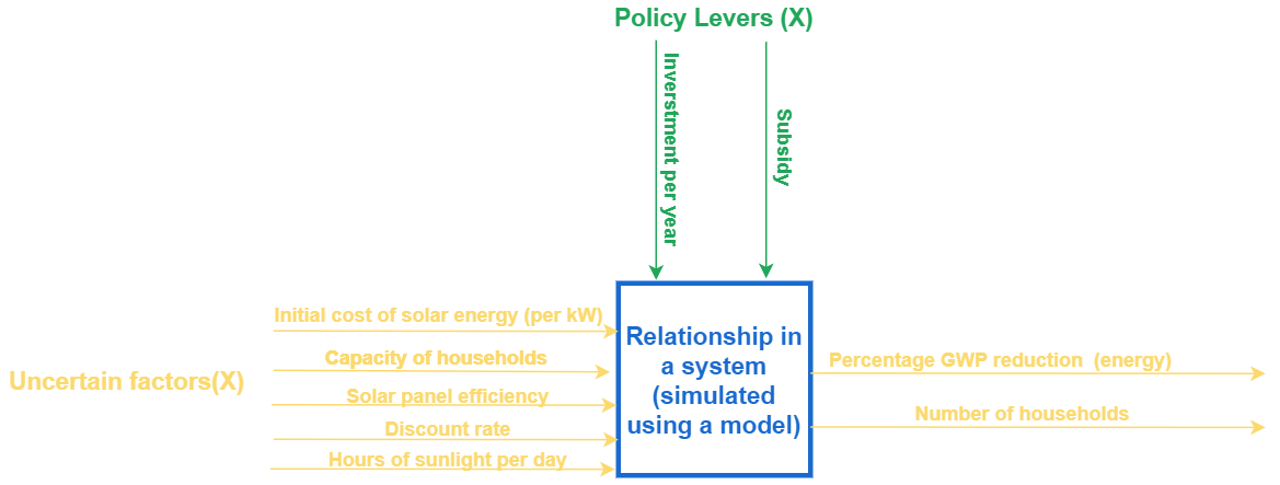
Say we want to use the EMA workbench to analyze how greenhouse gas (GHG) emissions can be reduced by installing solar panels on residential rooftops. Many governments are encouraging households to install solar panels by subsidizing the purchase of solar panels or by buying surplus energy directly from households. Let’s assume that the government invests a certain amount in these subsidies every year.
The government can decide what percentage of the cost of a panel it will cover with its subsidy. The total amount of electricity generated by solar panels and the resulting reduction in GHG emissions is impacted by other uncertainties, such as the initial cost of solar energy, the average number of panels a household can install, the efficiency of solar panels, technological developments in the photovoltaic industry (discount rate), and how many hours of sunlight there are in a day. These factors and others will eventually determine how much of a reduction in GHG emissions can be achieved, and how many households can use the subsidies on solar panels.
Setting the uncertainty ranges and doing the model runs
To use the EMA workbench, we first specify a range of values for uncertain factors in four different policy intervention scenarios. The four policy scenarios represent extreme values of the two sets of policy levers.
- Under policy 1, the subsidy is set at 20% and the government invests 1 million euros per year for a period of 10 years.
- Under policy 2, the government invests 10 million euros per year, while the subsidy rate remains unchanged, at 20%.
- Under policy 3, the government invests 1 million euros every year, while the subsidy is set at 60%.
- Under policy 4, the government invests 10 million euros per year, while the subsidy is set at 60%.
These uncertainty ranges are entered into the tool (see table below for the ranges we used in the case study; factors marked ‘X’ are background processes and ‘L’ are policy levers, or foreground processes).
Next, EMA workbench does a pre-specified number of model runs. Analyses of the results of each scenario helps us understand the impact of each policy and of the uncertain factors on the resulting metrics.
| Variable | Range | Unit | Explanation |
| Initial cost of solar energy (X) | [0.5,2] | €/kW | Cost of panels is measured in €/kW |
| Average number of panels a household can install (X) | [1,5] | kW | Depends directly on the surface area of households |
| Efficiency of solar panels (X) | [0.15,0.2] | fraction | Depends on the material of the panels |
| Hours of sunlight per day (X) | [5,10] | hours/day | |
| Discount rate for solar energy (X) | [0.03,0.07] | fraction | Factor by which solar energy becomes cheaper every year |
| Subsidy (L) | 0.2 and 0.6 | fraction | What fraction of the cost of a panel the government will cover with its subsidy. |
| Investment per year (L) | 106 and 107 | Euro | The amount of money that government invests in providing solar panel subsidies every year |
Two policies clearly outperform the others
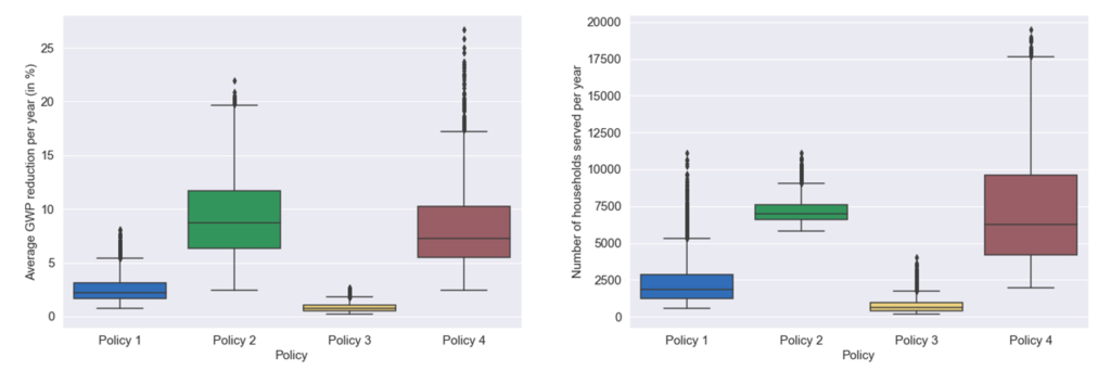
The results (see boxplots) show the following:
- Policies 2 and 4 are the most effective at both reducing the global warming potential (GWP) attributable to energy use and increasing the number of households that have solar panels.
- On average, reductions of around 9% and 8% in GWP attributable to energy use can be achieved with policies 1 and 3 respectively, up to 20% with policy 2, and up to 25% with policy 4.
- Around 7,000 households can take advantage of the subsidies under policies 2 and 4, whilst policies 1 and 3 only serve under 2,500 and 1,000 houses respectively.
Based on this analysis, it is clear that policies 2 and 4 outperform policies 1 and 3.
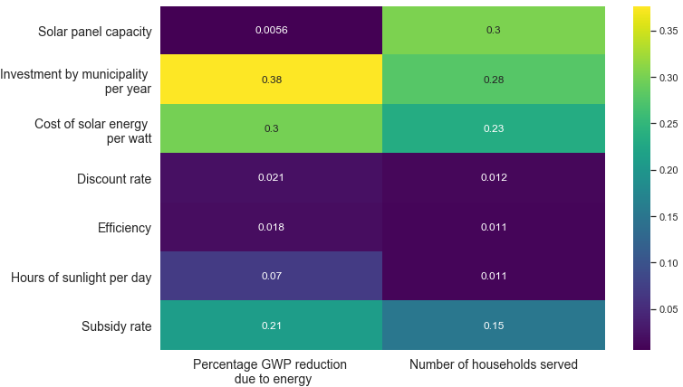
Seeing such a clear result is very valuable. However, it is also useful to understand the relative importance of different input variables, both foreground and background. That is what feature scoring does. The figure below shows how much the different input variables affect the two goals of reducing GWP and increasing the number of households benefitting from the subsidy.
Emission reduction is most influenced by the level of investment by the government, followed by the initial cost of solar power. These two aspects alone are responsible for 60% of the total reduction in GWP due to solar power. The number of households served depends equally on the capacity of households (i.e. the number of solar panels a household can afford) and the level of investment by the government.
If you want to use the EMA workbench, or dig deeper into the tool, take a look at this documentation. Although this case study was fairly simple, we hope we’ve shown the benefits of computational experimenting with the EMA workbench. Especially when you compare it to other uncertainty analysis methods which allow specifying one model at a time, you can see how much time the EMA workbench can save.
Ruchik Patel
Ruchik worked for PRé as an Analyst in 2020-2021. He worked on pioneering biodiversity footprinting projects for a variety of clients in the financial sector. Furthermore, he applied his programming skills to automate data collection and the presentation of results. His area of expertise also includes developing online tools with PRé’s software package SimaPro.